Step-by-Step Guide to KEGG and GO Analysis of Differentially Expressed Genes Using R-scripts and DAVID
gene_x 0 like s 1352 view s
Tags: genes, plot, R, KEGG, GO, pathway
Download the file WT_vs_K3R_sig_GO_top5.txt
Step-by-Step Guide for KEGG and GO Analysis from Differentially Expressed Genes:
-
Identify differentially expressed genes: Using the significance threshold (p-value <= 0.05, log2foldchange <= -0.58 and log2foldchange >= 0.58 or log2foldchange <= -2 and => +2), filter the significantly differentially expressed genes from your dataset.
-
Perform KEGG and GO enrichment analysis: Use a reliable tool like DAVID (https://david.ncifcrf.gov/) to perform KEGG pathway analysis and GO term enrichment based on the significantly differentially expressed genes. Export the enrichment results in text format.
-
Rank the enrichment results: Rank the KEGG pathway and GO term results using -log10(FDR) or -log10(p-adjusted) to better display the differences in values, especially when the values are too small to differentiate.
-
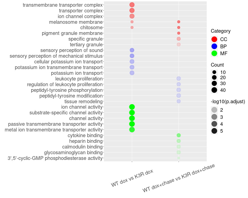
Visualize the enrichment results using R-scripts: Use the provided R-scripts to generate bubble plots for the KEGG pathway and GO term enrichment results.
Here's a detailed breakdown of the steps for visualization using R-scripts:
-
Install required R packages: Install the necessary R packages, such as ggplot2, for generating the bubble plots.
-
Load enrichment results: Import the text format output from DAVID or other web enrichment portals into your R environment.
-
Generate bubble plots: Use the attached R-scripts to create bubble plots for the KEGG pathway and GO term enrichment results.
-
Interpret and report the results: Analyze the bubble plots to identify the most significant KEGG pathways and GO terms associated with your differentially expressed genes. Include these findings in your research reports or publications.
library(ggplot2)
library(dplyr)
library(magrittr)
library(tidyr)
library(forcats)
mydat <- read.csv("WT_vs_K3R_sig_GO_top5.txt", sep="\t", header=TRUE)
mydat$GeneRatio <- sapply(mydat$GeneRatio_frac, function(x) eval(parse(text=x)))
#mydat$FoldEnrichment <- as.numeric(mydat$FoldEnrichment)
mydat$Category <- factor(mydat$Category, levels=c("CC","BP","MF"))
mydat$Comparison <- factor(mydat$Comparison, levels=c("WT dox vs K3R dox","WT dox+chase vs K3R dox+chase"))

#mydat$Description <- factor(mydat$Description)
#mydat <- mydat %>% mutate(Description = fct_reorder(Description, row_number()))
description_order <- rev(c("transmembrane transporter complex","transporter complex","ion channel complex","melanosome membrane","chitosome",  "pigment granule membrane","specific granule","tertiary granule",     "sensory perception of sound","sensory perception of mechanical stimulus","cellular potassium ion transport","potassium ion transmembrane transport","potassium ion transport",   "leukocyte proliferation","regulation of leukocyte proliferation","peptidyl-tyrosine phosphorylation","peptidyl-tyrosine modification","tissue remodeling",     "ion channel activity","substrate-specific channel activity","channel activity","passive transmembrane transporter activity","metal ion transmembrane transporter activity",       "cytokine binding","heparin binding","calmodulin binding","glycosaminoglycan binding","3',5'-cyclic-GMP phosphodiesterase activity"))
mydat$Description <- factor(mydat$Description, levels = description_order)

png("bubble_plot.png", 1000, 800)
ggplot(mydat, aes(y = Description, x = Comparison)) +
  geom_point(aes(color = Category, size = Count, alpha = abs(log10(p.adjust)))) +
  scale_color_manual(values = c("CC" = "red", "BP" = "blue", "MF"="green")) +
  scale_size_continuous(range = c(4, 10)) +
  labs(x = "", y = "", color="Category", size="Count", alpha="-log10(p.adjust)") +
  theme(axis.text.x = element_text(angle = 20, vjust = 0.5)) +
  theme(axis.text = element_text(size = 20)) +
  theme(legend.text = element_text(size = 20)) +
  theme(legend.title = element_text(size = 20)) +
  guides(color = guide_legend(override.aes = list(size = 10)), alpha = guide_legend(override.aes = list(size = 10)))
dev.off()
点赞本文的读者
还没有人对此文章表态
本文有评论
没有评论
看文章,发评论,不要沉默
最受欢迎文章
- Motif Discovery in Biological Sequences: A Comparison of MEME and HOMER
- Calling peaks using findPeaks of HOMER
- Kraken2 Installation and Usage Guide
- Why Do Significant Gene Lists Change After Adding Additional Conditions in Differential Gene Expression Analysis?
- Should the inputs for GSVA be normalized or raw?
- PiCRUST2 Pipeline for Functional Prediction and Pathway Analysis in Metagenomics
- Updating Human Gene Identifiers using Ensembl BioMart: A Step-by-Step Guide
- pheatmap vs heatmap.2
- Setup conda environments
- Guide to Submitting Data to GEO (Gene Expression Omnibus)
最新文章
- Risks of Rebooting into Rescue Mode
- 足突(Podosome)、胞外囊泡(Extracellular Vesicle)与基质金属蛋白酶(MMPs)综合解析
- NCBI BioSample Submission Strategy for PJI and Nasal Microbiota Study
- Human RNA-seq processing for Data_Ben_RNAseq_2025
最多评论文章
- Updating Human Gene Identifiers using Ensembl BioMart: A Step-by-Step Guide
- The top 10 genes
- Retrieving KEGG Genes Using Bioservices in Python
推荐相似文章
Processing RNAseq_2025_WT_vs_ΔIJ_on_ATCC19606
MicrobiotaProcess Group2 vs Group6 (v1)
